We have a listing of inbound purchases as recorded in our ERP which is distributed with an Excel workbook.
The workbook has a models sheet, a simple listing of open purchase line item details. The items are imported by FCL (container). There might be several dozen line items/SKUs in each FCL. Each SKU belongs to a product category. The business distributes about 50 product categories. Each FCL may have SKUs from several categories, but typically less than 4.
The second sheet is shipments which summarises the purchases line items by FCL which are tracked and other import admin stuff.
For each row on the shipments tab, one of the columns lists the product categories within each FCL
e.g.
Container . . . . . . . . CATs
OOCL123456789 . . PC4, PC3, PC6
The product categories within each container are listed in decreasing FOB value, though alphabetically would do.
I get this done with a pivot table from the model sheet by FCL by category, displayed by decreasing FOB. Concatenate the categories listed, bring the text value into the shipments tab with a VLOOKUP.
Bit clunky, but it works.
Am looking for an alternative, neater method to achieve an equivalent result with formulas if feasible.
I was looking at using something like UNIQUE and FILTER, but the unique values for each row/FCL need to be displayed in a single cell, not a dynamic column list.
Assuming that description makes sense, would anybody know a cunning way of achieving this?
Is there any way you can upload a sample file with the relevant sheets, either in Excel Online, Google Sheets, a shareable link to a file, etc.? It can have 100% fake data (as long as it’s in the same format).
Sorry, I read your description a few times and it was hard to make sure I understood it correctly. A sample file would be easier to understand, if it’s not too much trouble to make.
I’m not sure if I understood this right, but if you managed to get it into a format where the filtering is correct, but each row has a bunch of added columns for the categories, maybe you could hide those categories and TEXTJOIN() their values into a single cell.
It’d still be helpful to see an example file, though.
You’re welcome! If you need any further tweaks (like a different sort order), let us know. I’m not sure which of your current columns refer to the “FOB value”.
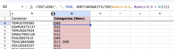
Here is the example spreadsheet with the new formula: ContainersV2.xlsx - Google Sheets (with some extra columns hidden to simplify the example)
In the “Shipment” sheet, column G has the formula:
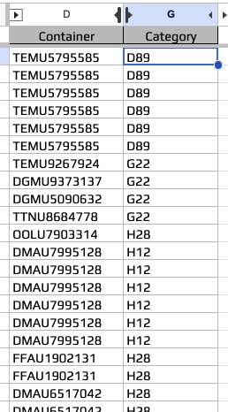
That points to the “Models” sheet, which has the same container IDs. Each row also has a category, and each container ID can have one or more rows/categories:
The formula just filters the Models!G:G by the matching container ID, extracts the UNIQUE() ones, SORT()s it, and then concats them all using TEXTJOIN(). No pivot table needed.
Where you might need a pivot, or a more complex formula, is if you wanted to sum up some other value to aid in sorting, i.e., calculating the sum of each container or category’s FOB value (still not sure which column that is) and then sorting the joined categories by that, per row in Shipment. It’s a lot simpler if you can live with just the alpha-numeric sorting that’s currently in place.