Next week, or the one after that, according to Elon Musk…
No earth shattering, but definitely a great idea. A lot of the interconnect real estate consists of power bumps, so moving them gives more room for I/Os and lets them be further apart.
Plus it would have helped with a weird bug we saw. One signal path on our processor would mysteriously rise in voltage, and cause an error. Nothing disastrous, it would just cause a reboot. It only showed up when you had the chip in a system, and the best test was letting the system sit at a prompt. It might show up in a few hours, it might show up in a few days.
It turned out there was some sort of coupling with this line and a power bump. We never could prove it, but when we rerouted the signal away from being under the bump the problem went away. Moving the power bump under the chip would have fixed this.
Since we’ve wandered from power requirements to comparisons, this:

And this was an iPhone 7.
(Seen on the wall of the the American Computer & Robotics Museum — in Bozeman, Montana, of all places.)
Unit analysis can be fun this way. Another unrelated example: gas mileage is measured in miles/gallon. But that’s a unit of inverse area. If we invert it to get ordinary area, what’s the meaning? It’s just the cross-section of a thread of gasoline that a car would have to “eat” as it goes down a road (usually, around a few hundredths of a square millimeter).
Getting back to the computation, 125 J is about the energy released when dropping a 30-lb barbell from a meter up. 15 pJ is roughly a single grain of pollen.
Yes, thanks for this, Dr Strangelove. I was not following the discussion at all, until you put it in these terms.
What additional storage do you mean? An SD card? Or files saved on cloud?
I’m thinking local storage - devices like phones, tablets, laptops and ultra-compact PCs that use SOCs often have one or more additional flash storage ICs and/or RAM, even if the SOC contains some.
Some interesting facts about the Univac 1. The power supply filter included a 1 farad capacitor–made up of 2000 electrolytics, 500 microfarads each. There were exactly 1000 adressable memory locations, each of which consisted of 12 bytes, 6 bits each. (“Byte” varied between 6 and 9 bits depending on the architecture–thus the French translation “octet” is misleading). But only 100 of these locations were accessible at any time–the other 900 were in a mercury acoustic delay tank; thus the machine really had only 100 memory locations, plus some registers. Programmers learned something called minimal latency coding, choosing memory locations designed to minimize the waiting time for the named location to be available. The lab I worked for wrote a program of 80,000 double words, about half were the logic needed to get the right routine in the machine at the right time. The main program was stored in a mag tape drive. The programming language could be best described as a hard-wired assembler. E.g. the word M356 was an instruction to multiply the contents of the memory location by the number in the multiply register and occupied 6 Bytes.
As someone mentioned above, the arithmetic was in binary coded decimal. But it was in what was called “excess 3”, meaning that, say a 2 was coded as binary 5: 101. The reason for this odd coding was that when an addition resulted in a binary carry, this meant the corresponding decimal carried as well. I guess this optimized something.
Ah, luxury!
The machine I learned to program on was an LGP-21, which was a transistorized version of the LGP-30 from about 1956. (The Computer History Museum has one.) No memory except for one accumulator - everything was stored on a disk, and there was a little round calculator to find where to place the next data element to minimize latency.
It did not use ASCII. Characters were coded in 6 bits, and the alphabet was arranged so that if you chopped off the least significant two bits you’d get the opcode. So Z was 000001, which was a Stop (0000) and Bring (load accumulator from memory, 0001) was 000101, B.
I never had reason to sort in alphabetical order, which would have been a nightmare.
HP calculators used a 4-bit byte, though they called it a “nybble”. And they had their own peculiar encoding for BCD, which also apparently occasionally shaved off one op, though IIRC theirs had low digits with the “correct” value but high digits offset.
Apparently early big iron like the Johnniac (40 bits) and IBM 701 (36 bits) used big words; smaller computers like the PDP-1 used smaller words. But what were the addressable, or otherwise relevant, “byte” sizes on these machines?
Knuth originally used 6-bit bytes in his books, but at some point (I guess when he changed his model example computer architecture to RISC) changed it to 8 bits.
Ref
it seems the addressing system was to either fullwords of 36 bits or half-words of 18 bits. What the 701 used for character encoding isn’t given, but I’d bet there are three 6-bit characters per halfword.
It’s unclear whether or how the characters within an 18-bit halfword might have been addressed individually.
CDC6600s had 60 bit words and 12 bit bytes, though other ways of looking at words had different sizes. Later Cybers also had 60 bit words, but I remember more of a six-bit byte architecture when I taught Cyber Assembly language when I was in grad school. Might be wrong - it was a long time ago.
Yeah, Cyber 170 series were much the same. Still had 6 bit chars, 60 bit words. The big change was moving from discrete transistors to 7400 series integrated logic. The overarching architecture was very similar.
My first two undergraduate years were spent on a Cyber 173. Then we got Vaxen. That was a big shift
From the wiki:
The Cyber-72 had identical hardware to a Cyber-73, but added additional clock cycles to each instruction to slow it down. This allowed CDC to offer a lower performance version at a lower price point without the need to develop new hardware.
Don’t tell me nobody tried to hack that!
PLATO ran on Cybers, and the computation for the four-color problem proof was done on them.
Though teaching one’s complement was a big pain.
This is neither here not there, but these guys built a 6502 out of discrete transistors:
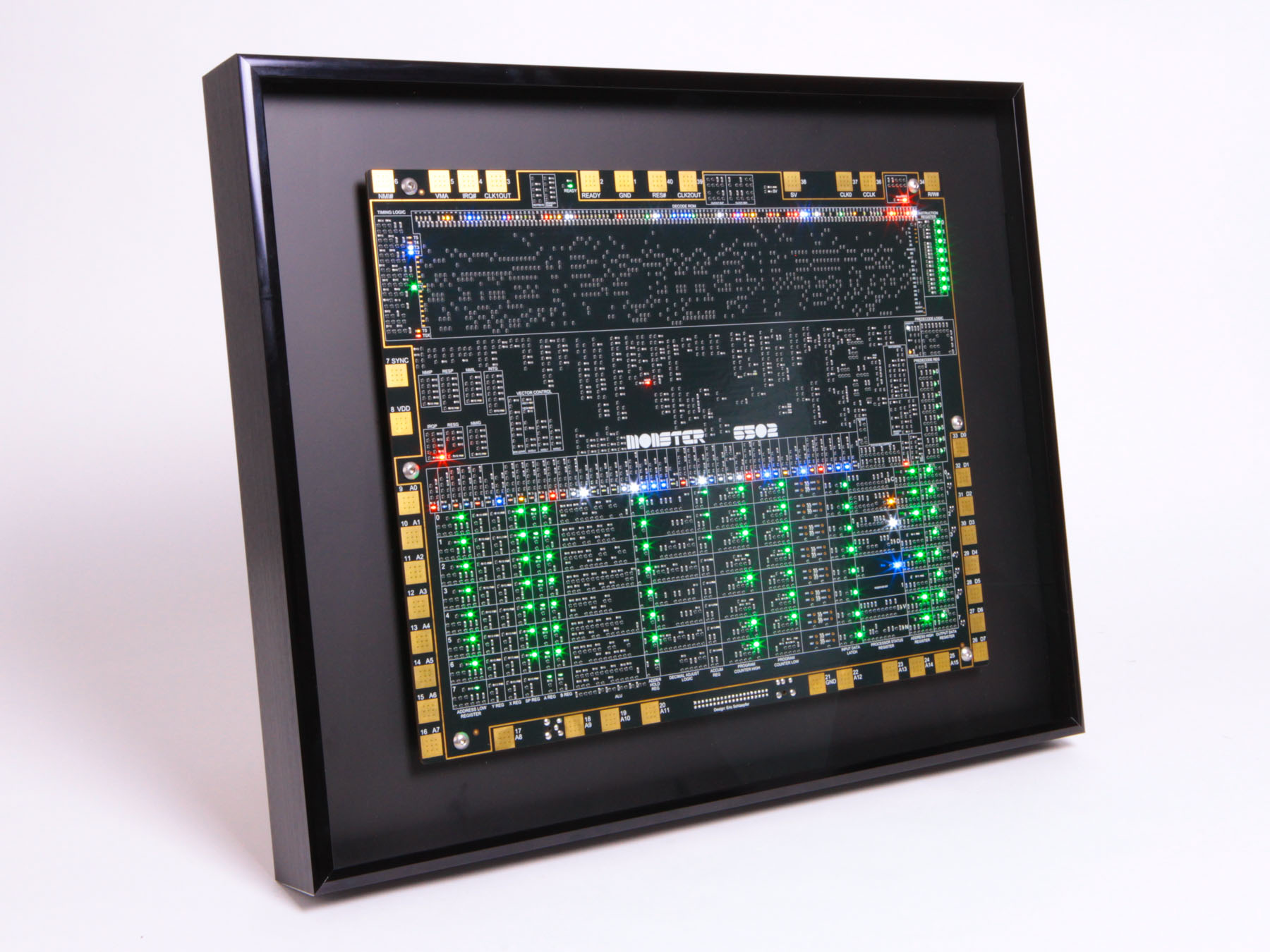
UNIVAC I might give it a run for its money, as it only runs at 50 kHz (though at 10 W).
I somehow don’t feel surface mount devices, discrete, or not has quite the same cachet. Pretty cool nonetheless.
The cordwood modules are lovely.

I have a selection of 6600, 173 and Cray 1 boards in my tiny collection.
I wonder what through-hole transistor packages could be used to make a version of that 6502 that still fits on a single board as ‘wall art’? TO-92 transistors only have a footprint of about 1/4 square cm, but component footprint is only part of the equation.
Also would TO-92 be retro enough, or would it have to be something in a metal can?
Hehe, the fifth question of the faq:
"#### Are you nuts?
Probably."