I will provide additional context below, but the TL;DR of my question is: where does that 0.00034% number come from: how is it derived or calculated, and what exactly does it mean?
The Wikipedia article on the normal distribution contains the offhand statement “Note that in a true normal distribution, only 0.00034% of all samples will fall outside ±6σ” (which I found by Control-F’ing the article), but with no citation or explanation. This number matches what @Exapno_Mapcase used and what appears in the link that @kenobi_65 provided.
However, this is a very different number from what I find on the table given earlier in that Wikipedia article, or from an online normal distribution calculator, for the probability of a normally distributed variable being more than 6 standard deviations away from the mean. (The table gives 0.000000001973 for this value, while the calculator gives 0.00000000198024, which is almost but not exactly the same.) This leads me to expect (naively?) that only 0.0000002% of all samples would fall outside ±6σ, not 0.00034%.
There obviously must be a difference between what the 0.0000034 is referring to/measuring and what the 0.000000001973 is measuring, but I can’t see what it is (although it’s entirely possible that there’s something obvious that I’m blockheadedly missing).
(For those wishing to refer to the original discussion, it starts at Post #22 of that other thread.)
I don’t even know whether I’m asking something simple and obvious, or deep and subtle. Can anyone explain to me where that number 0.00034% (or 3.4 per million, or however you want to express it) comes from?
As I understand it Sigma is a measure of uncertainty. It is an expression of the possible error in a measurement or calculation. The higher the sigma the smaller the possible error.
Which is to say, they cannot be 100% certain but they are so close at 5 or 6 sigma that they are very likely to be correct.
If you want to know how they arrive at this then the video below may help (14 minutes long):
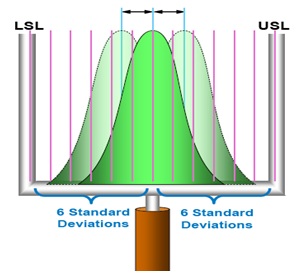
Basically if you assume your data is a bell curve, then the standard deviation is a fixed point on the curve (where 68% of the area under the curve is inside the region defined by the std dev point on the positive and negative X axis) that can be calculated. If you take that point and move it two “standard deviations” to the right you end up with sigma six (two as we are interested in the the “six” region with six standard deviations between minimum and maximum). You can go back to your bell curve and compute the area to the right of that (and to the left of the point on the opposite end of the graph) and you get your 0.00034%
One being an estimate of whether two distributions are different, the other being an expression for the number of outliers beyond a given distance from the mean.
Though in a business context I think this is what it is defined as. As in you should aim for only that tiny percentage of defective products to pass your QA process and end up with the customer.
I’m familiar with the basic ideas discussed there. And note that it says “six sigma translates to one chance in a half-billion that the result is a random fluke”—which seems to support my 0.0000002% rather than the 0.00034%. So that doesn’t help me understand where the 0.00034% comes from.
Your image shows 12 standard deviations between minimum and maximum—six to either side of the center—which is what I thought “six sigma” should mean.
That is where the name comes up a great deal. A business management religion that sort of claims to guarantee such defect rates. Software in particular. But one sees it all over the place.
I knew people at Motorola, which is where it came from, and the reality was not exactly what was claimed.
Judging from that same Wikipedia article some actual statics nerds also think there’s a big dollop of gobbledygook there
The statistician Donald J. Wheeler has dismissed the 1.5 sigma shift as “goofy” because of its arbitrary nature.[48] Its universal applicability is seen as doubtful.
The 1.5 sigma shift has also become contentious because it results in stated “sigma levels” that reflect short-term rather than long-term performance: a process that has long-term defect levels corresponding to 4.5 sigma performance is, by Six Sigma convention, described as a “six sigma process”.[9][49] The accepted Six Sigma scoring system thus cannot be equated to actual normal distribution probabilities for the stated number of standard deviations, and this has been a key bone of contention over how Six Sigma measures are defined.[49] The fact that it is rarely explained that a “6 sigma” process will have long-term defect rates corresponding to 4.5 sigma performance rather than actual 6 sigma performance has led several commentators to express the opinion that Six Sigma is a confidence trick.[9] Six Sigma - Wikipedia
The normal probability distribution function (PDF) has a nice explicit solution for its value as a function of the distance from the mean:
In discussing six-sigma concepts, you are dealing with the evaluation of the area under some portion of the normal PDF. This is an integral known as the cumulative distribution function (CDF):
While the normal PDF function is simple to evaluate analytically, the CDF is an integral that doesn’t lend itself to analytical evaluation. Instead, you have to use a numerical method to arrive at an approximation: The simplest version of this process is that you divide the area of interest under the curve into vertical rectangular strips, calculate the area of each strip, and add them all up to arrive at an approximation of the total area.
As that page shows, there are a variety of methods you can use to improve the accuracy of your approximation, although they all impart a computational effort requirement. The simplest way to improve accuracy is to make your vertical strips narrower and use more of them, but this also imposes a computational effort requirement. Whether you’re using Excel, an online calculator, or a handheld calculator, any of these programs/devices will be using some sort of approximate numerical integration scheme to spit out an answer for you, each with its own choice of compromise between giving you an accurate answer and a timely answer. The answers you’ve found from your tables are off by maybe a couple of parts per million, probably because whoever populated that table used one of the aforementioned calculators. An error of a couple of PPM is perfectly adequate for most purposes that most users might have in mind (e.g. anything between +/- 3 sigma), but not adequate for calculating anything out at six sigma, which is an extreme edge case.
If you’re familiar with Matlab or any other programming environment, you can create your own approximation of the CDF with your own tradeoff between accuracy and processing time. Use thousands or tens of thousands of vertical strips, use double-precision floating point variables, and so on. The longer you’re willing to wait for a result from your program, the more accurate your result can be.
Since the PDF uses a square root in a couple of places, it should be pointed out too that any square root you get from any calculator is also an approximation arrived at via a numerical method:
So you can likewise craft your CDF program to use one of these methods to calculate a square root to whatever accuracy you want for use in the PDF function.
Thanks for your answer, @Machine_Elf, but it doesn’t help me. I think that everything in your post is stuff I already know (though it may be helpful for others). It’s just that, as far as I can tell, the method you describe gives the value that I already thought it should be and not the value that @kenobi_65’s link and the statement “only 0.00034% of all samples will fall outside ±6σ” seem to say it should be.
Looking back at the other thread, I think what happened is that your link to the Wiki page didn’t pop out for me so I didn’t click on it and hence was just baffled by what you meant. Looking at it now, I see your concern. When I was googling for the six sigma percentage that didn’t come up; all I saw was the 0.00034% figure.
It’s a great joke on all of us if Motorola (and later GE) fudged the numbers to use the alliterative six sigma as an alliterative and unforgettable promotional tool rather than the correct but nerdy 4.5 sigma or whatever. I was just posting in another thread about the way common language often confounds scientific precision; this is a nifty example.
A friend of mine told me that he and Bill Smith (the originator of Six Sigma at Motorola) were friends, and one night he and Smith got drunk together, and Smith broke down and told him the whole thing just kind of got away from him. As I recall, he said something like “why would anybody do this? It’s just fucking stupid!”
This is now fourth-hand information, and my friend probably told me this a good 20 years ago, so…
Sadly there is a constant demand for magic bullets to make difficult problems go away. Six Sigma is just one of many. They save having to think. And even better, they include metrics that managers can use to get promoted or better pay.
Of course this demand also open opportunities for other companies to offer training and consulting in the magic process. At eye watering prices. But all very attractive to mangers, as they outsource the effort needed to get their company on the magical path and passing all the metrics that clearly show how fabulous a job he is doing.
How utterly bizarre. As best I can tell, not only did they introduce a 1.5 sigma shift, but they “forgot” to make it a two-sided integral. Doing the math via Wolfram Alpha:
For 6 sigma, it produces 1.97*10^-9, as expected (note that I folded the 2x into the formula).
Doing the same for 4.5 sigma:
That gives 6.79*10^-6, which is double the 3.4 ppm from the Six Sigma page. It’s like they forgot that a normal distribution has two sides.
I stared at it a bit before realizing what was going on, thinking maybe the 1.5 sigma shift was an approximation or something. But given that it’s exactly half the right amount, I’m pretty sure they just screwed up the integral.
How fitting that a program that might as well be a cult would be built on an error.